Cardiac Output 2

Introduction

In this document we will continue to look at how the body controls cardiac output. But first a bit more on venous blood return and the supplementary pumps of the CVS.

Venous Return Mechanisms

Circulation through the blood vessels of our bodies, as you have seen, depends upon more than the power stroke (ventricular systole) of the heart.

• The pulmonary artery and the aorta store some of the pumping energy of the heart and release it during ventricular diastole to keep arterial blood moving while the ventricles fill (~60 % of the cardiac cycle is devoted to filling the ventricles).
• The skeletal muscle pump (really pumps, since there are lots of them), provides most of the motive power for venous return from regions of the body below the heart.
• We went over the mechanics of the skeletal muscle pump last class, but here is a nice review.
• Notice that activity (moving about) is not required for the skeletal muscle pump to work in the legs.

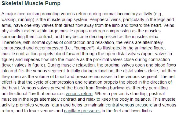
Text and graphic courtesy Richard Klabunde.

Venous Return in Paraplegics. Previously, a student asked what happens when a person loses the ability to contract muscles in the lower body.

• Loss of the ability to move lower limbs impairs the ability of the body to return blood from the legs to the heart.
• Edema (tissue swelling caused by accumulation of fluid) commonly results.
• Venous return can be improved by elevating the lower limbs and using compressive stockings (see this link).  The paper at this link demonstrates in greater detail how paraplegia impairs venous return.
• Why does any blood return from lower extremeties in a paraplegic individual? The answer to this is yet another pump!

Respiratory Activity (Abdominothoracic or Respiratory Pump) Respiratory activity influences venous return to the heart. Respiratory activity affects venous return through changes in right atrial pressure, which is an important component of the pressure gradient for venous return.  Pressures in the right atrium and thoracic vena cava are very dependent on intrapleural pressure (Ppl ), which is the pressure within the thoracic space between the organs (lungs, heart, vena cava) and the chest wall.  During inspiration, the chest wall expands and the diaphragm descends (see animated figure).  This makes the Ppl become more negative, which leads to expansion of the lungs, cardiac chambers (right atrium [RA] and right ventricle [RV]), and the thoracic superior and inferior vena cava (SVC and IVC, respectively).  This expansion causes the intravascular and intracardiac pressures (e.g., right atrial pressure) to fall.  As right atrial pressure falls during inspiration, the pressure gradient for venous return to the right ventricle increases.  Text and graphic courtesy Richard Klabunde.

To summarize the above: the same muscle movement that leads to inspiration during breathing creates a negative pressure for a brief time in the right atrium of the heart. This enhances the pressure gradient between the blood of the lower extremeties and the right atrium, drawing some blood up the inferior vena cava.

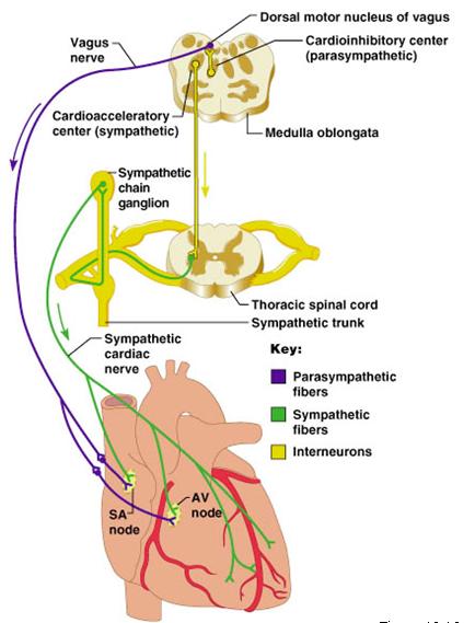
Back to Cardiac Output

As you saw last time, the heart achieves its variable output by altering both the heart rate (HR) and the stroke volume (SV):

CO = HR * SV

The specific mechanisms used to increase CO include:
 

Increased preload (preload = EDV) in combination with the Frank-Starling mechanism. This results in an increased force of contraction and increased SV.

Arrows indicate typical resting values (EDV = 120 ml, dead volume = 50 ml, SV = 70 ml).

Autonomic nervous system control of afterload (i.e., peripheral resistance). By relaxing the smooth muscles in the arterial tree, the size of the lumen increases, average velocity is decreased, and losses to friction decrease as well.

This graph represents what happens to the above curve if you reduce afterload (top curve) or increase it (bottom curve).

Autonomic (sympathetic only) nervous system control of contractility of the general myocardia.  Contractility is also called inotropy.  This increases or decreases the sensitivity of myocardia to the current passing through the heart (increasing or decreasing the speed of contraction).

The autonomic nervous system regulates the time delay of the AV node (this is a fairly minor mechanism).  Autonomic nervous system also regulates the SA node depolarization rate (i.e., heart rate). This causes the rate of depolarization of the SA node to change.

Courtesy Howard Medical School

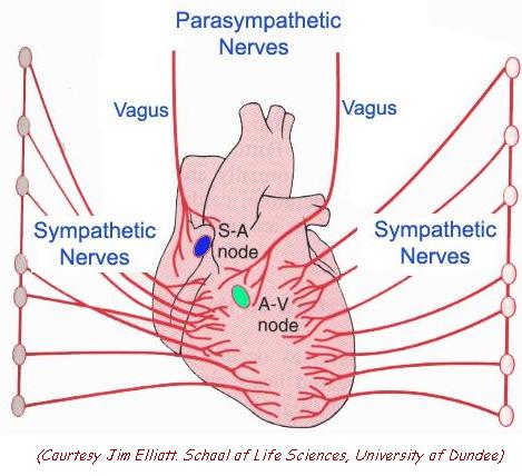
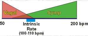
Heart Rate (HR)
 

Although resting human heart rate is ~60-80 bpm, the actual intrinsic periodicity (intrinsic rate of depolarization) of the SA node is ~100-115 depolarizations per minute.

The first 4 figures and the following quotes courtesy of Richard E. Klabunde, Ph.D

• Normally, at rest, there is significant vagal tone on the SA node ("tone" refers to the degree of nervous control; at rest, the vagus nerve is continuously inhibiting the rate of SA node depolarization).
• "For heart rate to increase above the resting rate, there is both a withdrawal of vagal tone and an activation of sympathetic nerves innervating the SA node. This reciprocal change in sympathetic and parasympathetic activity permits heart rate to increase during exercise".

Before we look more closely at stroke volume, let's look at the mathematical relationship that dictates what stroke volume will be: the Bernoulli equation.

Here's the frictionless Bernoulli equation:

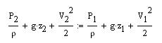
where P = pressure, z = elevation, V = velocity, and rho = blood density.

Each term in the equation has units of m²/s².

• As soon as we multiply each term by the mass (kg) of the fluid in question, the units of each term become kg*m²/s² , otherwise known as Joules.
• All that the Bernoulli equation is really stating is that energy is conserved from place to place along the path of fluid flow.

In the above equation, P_vent is affected by preload/F-S and by contractility, while P_aorta (really, the P of the entire arterial tree) is affected by adjustments in afterload.

Volumtric blood flow out of the left ventricle then comes from the product of the average velocity times the cross sectional area of the opening between the ventricle and the receiving artery.

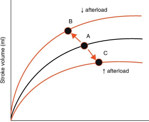
Afterload Adjustment to Compensate for Increased Cardiac Output

Changes in afterload are mainly proportional to changes in arterial cross sectional area and changes in blood velocity.

• Afterload, in unregulated arteries, will increase as cardiac output increases. The increased velocity of the blood through arteries increases friction, thus increasing back pressure in the arterial tree.
• The increased volume of blood in the arteries stretches the smooth muscle layer. Stretching smooth muscles causes them to contract, which could lead to vasoconstriction, which would also increase back pressure even more.
• These results are largely counteracted, however, by combined effects of the autonomic nervous system and local physiological responses which relax the smooth muscles in the arterial walls (vasodilation).

Inotropy is synonymous with contractility. Heart muscle cells are unique among muscle cells in that stimulation by the autonomic nervous system (sympathetic) can increase the speed of the myocardial responce to the arrival of a current. Skeletal and smooth muscles (the other muscle cell types found in the body) cannot do this.

If our heart rate is 60 bpm, then each complete cardiac cycle (diastole + systole) takes about 1 second. Since ventricular diastole is about 60% of the cycle, that allows about 0.6 s for the ventricle to fill and 0.4 s for ejection.

Now, let's get active: our heart rate goes up to 120 bpm. Each cycle is now only 0.5 s and filling/ejection must be accomplished in just half the time (0.3 s for relaxation + filling and 0.2 s for contraction and ejection).

• If the muscle cells contract more quickly, what subphase can the cardiac cycle pass through more quickly?
• And (as mentioned above) contractility also increases the maximum pressure generated during systole. Do you understand why this is true?

Stroke Volume, Heart Rate, and Cardiac Output

Definitions of Activity Levels. In a mathematical model created by graduate student Bruce Johnson, (a more sophisticated version of the cardiac model you did in biosimulation), activity levels are divided into a number of categories. These are summarized below for an average young male.
 

These activity levels are used in the figures, below.

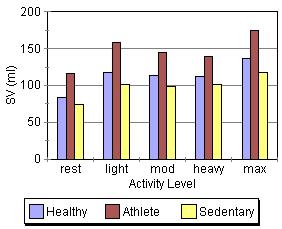
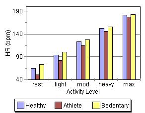
Activity, Conditioning, and Cardiac Output. The ABE CVS model was used to generate the stroke volume, heart rate, and cardiac output predictions shown below.
 
 

These graphs, at first glance, seem to contradict some of the things mentioned above (If changes in preload/F-S, contractility, and afterload change stroke volume, why are the stroke volume graphs nearly flat across all activity levels while cardiac output and heart rate show a steay increase?).

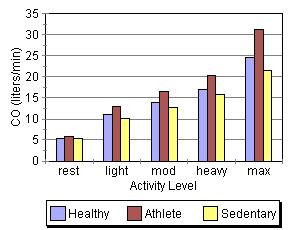This apparent paradox is resolved when you recall that the time available for filling and ejection is greatly reduced as heart rate increases. The effect of preload/F-S, contractility, and afterload changes is precisely why we can hold SV constant (or show a slight increase) even though the time available for systole and diastole is reduced by about two thirds across the range of the graphs. This is quite a remarkable and accounts for how a tripling of HR can result in a 500% increase in cardiac output!

Another interesting thing shown in the graphs is the role of conditioning in cardiac performance. Athletes show the greatest increase in cardiac output despite having the lowest heart rates. Much of their superioer perfomance is due to larger stroke volumes, which are an artifact of conditioning.

The Pressure-Volume Relationship
 

You have seen that left ventricle pressure and volume can be plotted against time.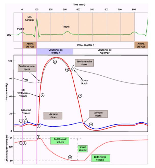

It is also useful and very instructive to plot them against each other.
 

If we do, we get a loop that just keeps going around and around.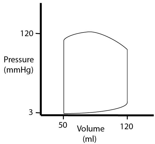

During the filling part of diastole, we see the left ventricle filling at low pressure. As volume increases, the compliance of the heart wall causes pressure to increase.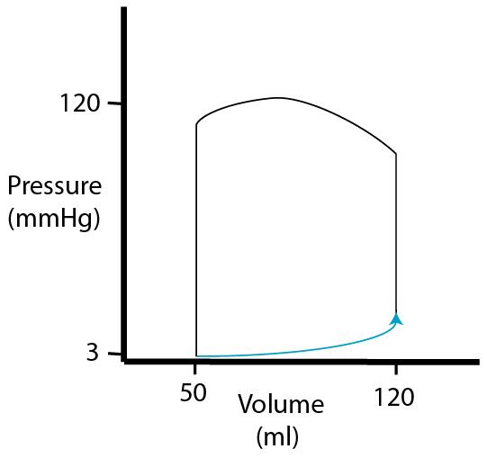

At the beginning of ventricular systole, pressure increases with no change in volume (hence the vertical line, isovolumic contraction). Why does volume remain constant?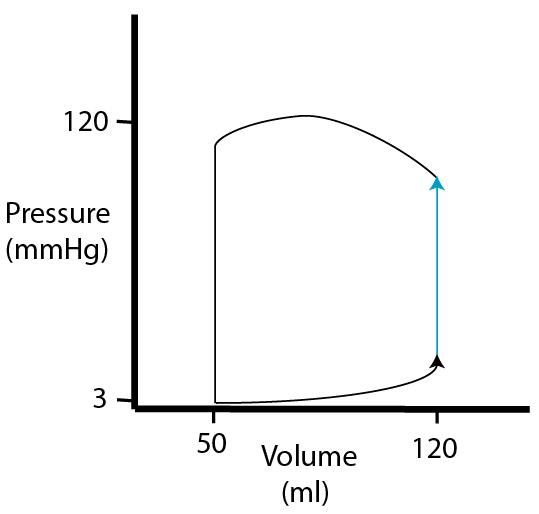

During the ejection phase of systole, the tension of the ventricular muscle cells first continues to increase and then remains constant (pressure decreases because volume decreases).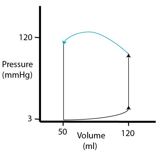

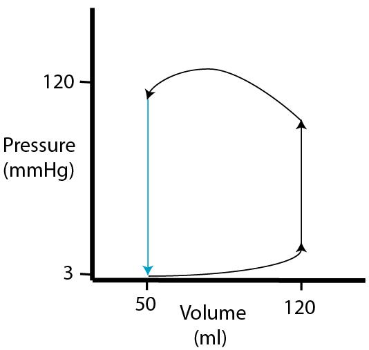
Finally, during the first sub phase of diastole, pressure drops with no change in volume (isovolumic relaxation).

As mentioned, stroke volume is EDV minus ESV. Stroke volume and the P-V loop will remain constant as long as activity level remains unchanged.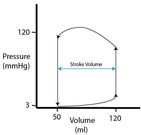

Some More Detail About these Plots

So now we have a loop that goes around and around as a ventricle undergoes systole and diastole. Let's look more closely at the shape of the plots.
 

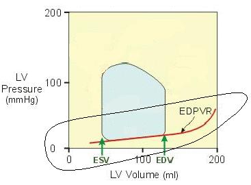
In the figure at right, "EDPVR" stands for "end diastolic pressure-volume relationship. "ESPVR" stands for "end systolic pressure-volume relationship. Let's start with EDPVR.

Image 6

The Bottom of the PV Loop (EDPVR)
 

You've seen the first graph at right before. It's compliance (for veins and arteries). If we reverse the axes, we have V on the x-axis and P on the y-axis (as in the P-V plots). Laid out this way (with the axes reversed), this relationship is called "elastance." Elastance is the inverse of compliance.

Image 7

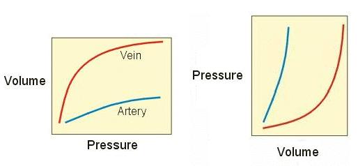Notice the shape of the elastance curve (especially the red one). Does it remind you of the EDPVR line? That's because they show a similar property in both blood vessels and ventricles: as you fill them up, pressure increases. The pressure change, in both cases, is a lot like the pressure change that you see when you blow up a balloon: it's due solely to the stretching of the walls (there is no active contraction going on).

Further, the amount that pressure increases depends upon where you are in the plot.

What is the significance of this plot?
 

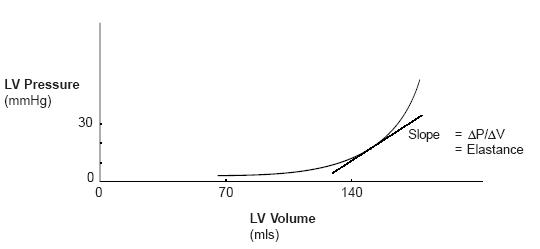
The graph at right shows ventricular elastance. Notice that the graph shows only a modest rise in pressure at lower volumes (dP/dV is small). Only when volumes become larger do we see that the graph turns upward (dP/dV increases).

Image 8 Courtesy of the Anesthesia Education Website.

The significance of this to the heart is two-fold.
 

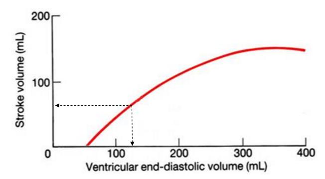
First, recall that the Frank-Starling mechanism results in increased force of contraction as myocardia are stretched during filling: the greater the stretch, the greater the force of contraction. But this relationship does not go on forever. It is possible to over-stretch the myocardia. If that were to happen, increased stretch would decrease force. In the graph at right, this is illustrated by the turn down in tension when myocardia are over-stretched.

Image 10

In a healthy heart, this does not happen. The increase in elastance at the far right of the curve becomes a barrier that prevents over-stretching.

Image 9

A second significant aspect of this curve is that increased elastance (hypertrophy, increased dP/dV) usually accompanies aging and can occur in certain heart pathologies. This causes the EDPVR curve to shift left, making the heart harder to fill. This is one cause of the decreased cardiac output in older people and those experiencing certain types of heart disease.

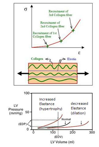
Why does stretching of the heart wall have a characteristic curved shape?
 

There's no magic involved. The upward curve in EDPVR is due to collagen and elastin in the heart walls):  As the heart walls stretch during filling, elastin first resists, causing a more or less linear pressure increase.  Collagen molecules having different degrees of looping are sequentially recruited (first the least looped, then those that are more looped).  As each is stretched straight, in turn, it contributes additional resistance to stretching.  In this way, the curvature of the P vs V curve during filling becomes more pronounced. The bottom graph in the figure at right shows normal elastance and two pathological conditions: decreased and increased elastance (dP/dv).

Courtesy Technical University of Denmark

So now we understand where the bottom of the PV loop comes from. It tracks the ventricular elastance curve.  But where does the curve start? Does it start at the origin? No, it does not start at the origin.

Image 11

Starting the elastance curve at the origin would suggest that adding blood to an empty ventricle would result in a pressure increase. This probably would not occur. Rather, we would expect a measurable increase in pressure with filling to occur somewhat to the right of the origin. We call this point Vo ("unstressed volume") in a PV plot. You will see its significance later.

The Top of the PV Loop
 

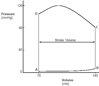
The vertical sides of the loop make sense because we know about isovolumic contraction (line BC) and isovolumic relaxation (DA). Why does the top of the loop look as it does? Answer: The shape of the top of the loop looks as it does because the peak tension of the myocardia (the point where all the muscle cells are fully contracted) occurs between C and D.  Recall that the cardiac cycle moves counter clockwise around the P-V loop and the bend to the left after C occurs because ejection has begun (volume is decreasing). If the myocardia reaches peak tension at or before C, pressure would drop all the way through ejection as the volume of blood in the ventricle decreases. If the myocardia tension continues to increase all the way to D, then pressure would increase all the way from C to D. The increase in pressure to a point between C and D followed by a decrease to D indicates that myocardia reaches peak tension between C and D. It is thought that once peak tension is reached, it is maintened all the way to D, with the drop in pressure being due to to continued ejection of blood into the aorta (think water balloon with a leak).

Image 12

The Usefulness of PV loops

We've gone to quite a bit of trouble to generate and understand P-V loops. A logical question is why bother? It turns out that P-V loops are almost the only way to observe and understand how the Frank-Starling mechanism, and changes in contractility and afterload effect cardiac performance and behavior. They are also good tools for identifying and understanding a variety of heart pathologies. More on this in the next class.

A bit more on heart rate changes and reinnervation of transplanted hearts (this is FYI only)

"Heart transplant recipients can exercise and are encouraged to exercise to improve the function of the heart and to avoid weight gain. However, due to changes in the heart related to the transplant, patients should speak to their doctor or cardiac rehabilitation specialist before beginning an exercise program. Because the nerves leading to the heart are cut during the operation, the transplanted heart beats faster (about 100 to 110 beats per minute) than the normal heart (70 beats per minute). The new heart also responds more slowly to exercise and doesn't increase its rate as quickly as before." MedScape Today

We can conclude from the above that parasympathetic reinnervation is not expected to occur. There appears to be good evidence for at least some sympathetic reinnervation and perhaps, in some cases, some parasympathetic reinnervation (but perhaps not connected to the SA node): "After heart transplant (HTX), the heart is completely denervated. While sympathetic reinnervation is likely to occur, there is conflicting evidence regarding parasympathetic reinnervation" Echocardiography, Volume 23 Issue 5 Page 383-387, May 2006

"Chronotropic incompetence [i.e., the inability to change heart rate] is considered to be the main limiting factor of the functional capacity of heart transplant recipients." J Am Coll Cardiol, 1999; 33:192-197

"The reduction in peak oxygen consumption, particularly during the first 2 years, appears to be related in part to chronotropic incompetence. Late after transplantation the heart rate response to exercise is greater and the decline in heart rate after exercise faster, suggesting possible autonomic reinnervation in some patients."  J Heart Lung Transplant. 1996 Nov;15(11):1075-83.
 

Finally, from the book Exercise and Sports Cardiology (published 2000):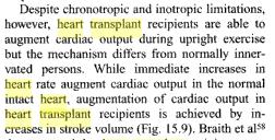

What can we conclude from the above? For most heart transplant patients, reinnervation is probably quite limited and CO increases are mainly due to the F-S mechanism and perhaps to reduction in peripheral resistance (afterload). Some reinnervation cannot be ruled out, however, suggesting that inotropy (rate of contraction) changes may also be possible, particularly some time after the transplant.
.